Example-Analysis

library(Morefi)

Morefi

Shield:

Morefi: Example Analysis

This is a methodological package developed in R for analyzing the submitted article:

Aguirre-Villaseñor, H., Morales-Bojórquez, E., Cisneros-Mata (FISH13711). Biometric relationships as a fisheries management tool: A case study of the bullseye puffer (Sphoeroides annulatus. Tetraodontidae). Fisheries Research.

In fisheries monitoring, body length is the most commonly measured parameter because it is quick and easy to obtain. In contrast, measuring weight requires a level and stable scale, which can be difficult to secure in field sampling. Biometric relationships are crucial in fisheries biology. When accurately calculated, these relationships can be very useful for management purposes, especially for estimating an organism’s total length or weight based on other body measurements.

Many species are marketed through artisanal fishing in various commercial forms. However, there are currently no biometric relationships that allow for predicting live weight (the total weight of the fish) from the different categories of landed weight, such as fillet weight, gutted weight, or frozen weight.

The objective of this package is to provide quantitative analysis for various morphological relationships that help predict: a) the expected live weight of different landed weight categories, b) the expected fillet yield from various commercial presentations, and c) testing the suitability of fillet yield as a reference point in managing the target species.

For this purpose, some functions and a vignette were created to explain the process step by step. Its implementation streamlines the methodology and enhances the clarity and impact of both the results and graphical presentations (tables and figures are personalized).

The functions included in the Morefi package enable the evaluation of length-length, weight-weight and length-weight biometric relationships using data that exhibit high variability and do not meet the assumptions necessary for adjustment via least squares. Given this variability, a robust regression method is employed for analysis. The “robustbase” package (version 0.99-2) was utilized to fit robust regression models, using the functions lmrob() for linear and nlrob() for non-linear regression (Maechler et al., 2024).

Installation

You can install the development version of Morefi from GitHub using one of the following options:

Using the pak package

# install.packages("pak")
pak::pak("Macrurido/Morefi")

or using the devtools package

library(devtools)
install_github("Macrurido/Morefi")

Data available in the package

To showcase the functionality of the Morefi package, the two data sets from Aguirre-Villaseñor et al. (Submitted) are included.

Bullseye puffer measures

To demonstrate how the package functions, we utilize the dataset botete, containing 1,397 fish across 7 variables: the total length(LT), standard length (SL), body trunk length (LB), total weight (WT), body trunk weight (WB), and fillet weight (Wfi) of the bullseye puffer (Sphoeroides annulatus), collected from the Eastern Central Pacific. In this dataset, the landing category is included in the “Fleet” variable, which is categorized as follows: 1 indicates Fresh, while 2 denotes Frozen-thawed.

To access the data file, the data frame is stored in an object, such as ‘mydata’.

mydata <- Morefi::Botete
str(mydata)
#> 'data.frame':    1397 obs. of  7 variables:
#>  $ LT   : num  21 22 12 21 12 28.4 29.3 34.8 31.7 31.5 ...
#>  $ LS   : num  17.3 17.6 10 17.3 10 23 24.2 27.5 25.5 26 ...
#>  $ LB   : num  17 15 10 15 8.5 20 20.5 27 23 24 ...
#>  $ WT   : num  189.1 213.4 33.4 236.7 36 ...
#>  $ WB   : num  115.6 86.7 15.4 100.4 18.9 ...
#>  $ Wfi  : num  50.7 55.5 6.9 65 9.1 ...
#>  $ Fleet: Factor w/ 2 levels "1","2": 2 2 2 1 2 1 2 1 1 1 ...

Bullseye puffer fish landings

A second dataset Botete_land, provided the Mexican fishing records of bullseye puffer landed on the Pacific coast in 2023 and their live weight corresponding live weight for each weight category (kg): total (WT), body trunk (WB) or fillet (Wfi), either Fresh or Frozen-thawed (SIPESCA, 2024).

To access the data file, the data frame is stored in catch.

catch <- Morefi::Botete_land
catch
#>          Category  Landed   Biomass    Pesos  Pesos_kg
#> 1        WT_Fresh  509354  509354.0  33079.5  41.49873
#> 2        WB_Fresh  449646  494610.6  58048.0  52.05232
#> 3 WB_Fresh_Thawed  361404  451755.0  37997.0  54.77369
#> 4       Wfi_Fresh   47990   95980.0  16485.0 112.83715
#> 5           Total 1368394 1551699.6 145609.5  50.97446

theme_papers()

The theme_papers() is created to standardize the graphic format, used as base theme_bw(). To showcase their design, this manual presents graphics in both their original format and the format created using the theme_papers().

To call the theme_papers() function use the following statement:

theme_papers <- Morefi::theme_papers()

Values to define for the examples

List: xseq

For the examples developed in this article, a list called x_seq is created to store the sequences of independent variables used in various models, specifically Total Length (TL) and Total Weight (WT). For each variable, the minimum and maximum values are established, as well as the bin range per sequence by.

# To round a number to the nearest 5
# Total length (LT)
    by <- 5
    LTmin <- floor(min(mydata$LT)/by)*by  
    LTmax <- round(max(mydata$LT)/by)*by

# Standard length (LS)    
    LSmin <- floor(min(mydata$LS)/by)*by  
    LSmax <- round(max(mydata$LS)/by)*by
    
# To round a number to the nearest 5    
# Total weight (WT)
    by <- 10
    WTmin <- floor(min(mydata$WT)/by)*by  
    WTmax <- round(max(mydata$WT)/by)*by

# Body trunk weight (WB)    
    WBmin <- floor(min(mydata$WB)/by)*by  
    WBmax <- round(max(mydata$WB)/by)*by
    
# List_x_seq    
List_x_seq <- list(LT= seq(LTmin,LTmax,by=1),
                   LS= seq(LSmin,LSmax,by=1),
                   WT= seq(WTmin,WTmax,by=10),
                   WB= seq(WBmin,WBmax,by=10))

List: modelos

A list that defines the variables that will be taken into account for the model.

modelos <- list (LTvs.LS  =  c(1,2),
                 LTvs.WT  =  c(1,4))

Morefi functions

The Morefi package includes functions that facilitate data analysis and ensure reproducibility of results. The functions for analysis are outlined below, followed by the functions for plotting.

Analysis functions

fn_ARSS()

The function fn_ARSS() perform the Coincident Curves Test, to determine if there are significant differences between the fitted curves for each database. It is based on the Analysis of the Residual Sum of Squares (ARSS) (Chen et al. 1992).

$F=\frac{\frac{RSS_{p}-RSS_{s}}{3\bullet \left( K-1 \right)}}{\frac{RSS_{s}}{N-3\bullet K}}$

$RSS_{p}= RSS$ of each regression fitted by pooled data, $RSS_{s}$ = sum of the $RSS$ of each regression fitted for each individual sample, $N$ = total sample size, and $K$ = number of samples in the comparison.

The residual sum of squares $RSS$ and the degrees of freedom $DF$ for each fitted regression are previously stored in the List_TCCT list. For each regression, the calculations are stored in a data frame T1, which is stored iteratively using a loop for in a list T.

Inside the function, the RSS and DF for the joined sample are calculated to perform the F test for two tails $\alpha/2$ . The decision criteria is performed: “*” if $p-value\le \alpha$ or “NS” if the $p-val\gt \alpha$ .

The function requires defining:

List_TCCT: A list with fitted regression results.
i: An integer value indicating the ith regression analyzed.
alfa: A numerical value that defines the significance level. The default number is 0.05.

The function return a data frame containing the results of the Coincident Curves Test stored in a list.

Example

The Total length (LT) - Total weight (WT) was estimated for the bullseye puffer Sphoeroides annulatus for landed categories: Fresh, Frozen-thawed (Frozen), Total (All sample) and Joined (sum of values of Fresh and Frozen). The Residual Sum of Squares (RSS) and the degrees of freedom (DF) are provided for each data source. In the table the first row displays the Analysis of Residual Sum of Squares (ARSS), the p-value (p), and the decision criteria for the ARSS test (Criteria).

In the table the first row displays the Analysis of Residual Sum of Squares (ARSS), the p-value (p), and the decision criteria for the ARSS test (Criteria).

The adjusted models show the following data: Fresh SSR= and DF= 742; Frozen SSR= 1280131.81 and DF= 651; and the total sample SSR= 6115874.53 and DF= 1395. Values are stored in the table Table_CC, this is stored in a list, and the name of each item is built with the acronyms of the model variables (e.g. LTWT).

Table_CC <- data.frame(matrix(NA,nrow=4,ncol=8))
Table_CC[1,1] <- "Lt-WT" 
Table_CC[,2] <- c("Fresh","Frozen","Total","Joined")
colnames(Table_CC) <- c("Model","Category","RSS","DF","ARSS","F-table","p-value","Criteria")

Table_CC[1,3] <- 4424418.33
Table_CC[1,4] <-  742 
Table_CC[2,3] <- 1280131.81
Table_CC[2,4] <-  651 
Table_CC[3,3] <- 6115874.53
Table_CC[3,4] <-  1395 

List_ARSS <- list(LTWT=Table_CC)

i <- 1

ARSS <- fn_ARSS(List_ARSS, i,  alfa= 0.05)

Table of the Coincident Curve Test.
Model	Category	RSS	DF	ARSS	F-table	p-value	Criteria
LT vs. WT	Fresh	4424418	742	0.0721	1.0921	0.05007	NS
NA	Frozen	1280132	651	NA	NA	NA	NA
NA	Total	6115875	1395	NA	NA	NA	NA
NA	Joined	5704550	1393	NA	NA	NA	NA

fn_dfa()

This function uses the augment() function from the broom package to extract the observed values of the independent variable (x) and dependent variable (y), along with the weights (wi), fitted values (fitt), and residuals (ei) from the summary of the fitted model. It then turns these components into tidy tibbles.

The function augment() does not provide the weights column for the lmrob() function. The function fn_dfa() contains a conditional statement that includes this variable in the output data frame of the linear adjustments.

In order to homogenizes the results, the columns names were renamed as “y”, “wi”,“x”,“fitt”,and “ei”.

An additional column has been included that codes errors using a scale based on weighted values: unweighted (u), weighted (w), and outliers (o) dfa$scale <- ifelse(df$wi < 0.25, "o", ifelse(df$wi<1, "w", "u")).

The function requires defining:

eq: Summary of the equation fitted.

Example

Using the biometric data from Morefi::botete, a linear relationship between Total Length and Standard Length (LT_LS) was established using the robustbase::lmrob function. Additionally, the relationship between Total Length and Total Weight (LT_WT) was fitted using the robustbase::nlm function, with an input y-value of a = 0.1 and a slope of b = 3.

For optimal functionality of fn_dfa(), the data frames used for fitting relationships must be formatted as tibble.

The first six rows of the table are displayed, based on the LT versus LS relationship results.
y	x	fitt	ei	wi	scale
17.3	21.0	17.174230	0.1257696	1.0000000	u
17.6	22.0	17.999109	-0.3991088	0.9914912	w
10.0	12.0	9.750324	0.2496758	1.0000000	u
17.3	21.0	17.174230	0.1257696	1.0000000	u
10.0	12.0	9.750324	0.2496758	1.0000000	u
23.0	28.4	23.278331	-0.2783310	1.0000000	u

The first six rows of the table are displayed, based on the LT versus WT relationship results.
y	wi	x	fitt	ei	scale
189.1	1.0000000	21.0	209.81549	-20.715491	u
213.4	1.0000000	22.0	242.19890	-28.798897	u
33.4	1.0000000	12.0	37.32321	-3.923211	u
236.7	1.0000000	21.0	209.81549	26.884508	u
36.0	1.0000000	12.0	37.32321	-1.323211	u
457.0	0.5098231	28.4	532.50610	-75.506104	w

`fn_freq()`

It is used as an internal function within fn_freqw().

The fn_freq() function calculates a frequency distribution of data using the cut() and table() functions from the R base. It produces a data frame that displays frequencies categorized by class interval.

Within the function, the non-cumulative absolute frequency is calculated for each user-defined class interval based on the breaks object. The breaks object must be defined outside the function by the user.

The attributes and examples of fn_freq() are detailed in the documentation for the fn_freqw() function below.

See also cut() and table() from the R base package.

fn_freqw()

The fn_freqw() calculate the percentage frequencies of weights by model adjusted using the robust regression approach. The function calculates the relative frequency distribution using the function fn_freq() from Morefi package. It returns a table with frequencies by class interval.

The breaks object must be defined. To incorporate the number of non-weighted values $(w_{i}=1)$ , a class interval “1” is added to the sequence inside the function.

The function requires defining:

df A vector of data values.
breaks A vector with class intervals.
right Logical, indicating if the intervals should be closed on the right (and open on the left) or vice versa.

See also Morefi::fn_freq; cut() and table() from the R base package.

Example

The weighted values were obtained from the summary of linear and power models fitted using robust regression and stored in dfa1 and dfa2, which were generated with the fn_dfa() example. In each data frame, the weighted values are stored in the column labeled “wi.”

The function fn_freqw() calculates the frequency of weighted values within a defined interval based on a weighted scale classification: unweighted $(w_{i}=1)$ , weighted $(1>w_{i}≥0.25)$ , and outliers $(w_{i}<0.25)$ . The weighted scale is stored in breaks.

Percentage frequencies of weights (wi) based on a weighted scale classification
	freq1	freq2
[0,0.25)	1.216893	3.364352
[0.25,1)	30.064424	27.057981
[1,Inf)	68.718683	69.577666

fn_xseq()

The function generates a data frame with a sequence for independent variable (including minimum and maximum values) and selects it according to the model.

The data frame should have the same column name as the dependent variable used in the fitted model.

Inside the function, the appropriate sequence is selected in function of model the mean Ymean, lower Ymin, and upper Ymax CI95% are stored in a table Table_Y

The function generates a data frame with a sequence for independent variables (including minimum and maximum values) and selects it according to the model.

Example

The objects modelos and List_x_seq were defined earlier in the section titled Values to Define for the Examples.

fn_intervals()

The function calculates a non-parametric confidence and predicted intervals using the function predFit() from the package investr (version 1.4.2).

The function requires defining:

xseq A vector with a sequence for independent variable.
eq Summary of the equation fitted.

The function return a data frame df with the xseq (x1), the fitted values for dependent variable (fit), the low and upper confident (IC_L and IC_U) and predicted intervals (IP_L and IP_U).

Example

fn_fyield()

The function calculates the fillet yield by dividing a defined weight reference point bm by the mean, lower, and upper confidence interval of 95% (IC95%) of the estimated fillet weight, respectively. These values are obtained from the list items l_intervals$CI returned by the function Morefi::fn_intervals().

If the analyzed regression has fillet weight as an independent variable, then values are calculated. An “if statement” is written for this propose.

Fillet yield was calculated for a sequence of the independent variable (including minimum and maximum values).

Inside the function, the mean (Ymean), lower (Ymin), and upper (Ymax) CI95% are stored in a table (Table_Y).

The function requires defining:

Example

fn_R2RV()

The function calculates a robust version of the coefficient of determination $R^{2}_{RV}$ using the Equation Summary values fitted with the robustbase::nlrob() function.

This is the consistency corrected robust coefficient of determination by Renaud and Victoria-Feser (2010) which allows for a possible correction factor a for consistency considerations.

Inside the function:

The vectors of observed (y1), predicted (yc) and weighted (W) values are obtained from the summary model (eq).

The value of the Weighted Estimate Average (ywea), the modified sum of squares for explained (SSEw), total (SSTw), and residual (SSRw) were estimated.

The correction factor value for consistency considerations a for 95 percent was also obtained from summary model (eq).

A vector with the robust version of the coefficient of determination R2wa and its adjusted value R2wa_adj were returned as a vector.

In the function, the following were estimated:

The Weighted Estimate Average $\overline{\widehat{y}}_{w}$ (called as ywea).

$\overline{\widehat{y}}_{w}=\left(1/\Sigma w_{i}\right)\times \Sigma w_{i} \widehat{y}_{i}$

The modified sum of squares explained SSEw $SSEw= \sum_{}^{}w_{i}(\widehat{y}_{i}-\overline{\widehat{y}}_{w}) ^2)$

In this function, the robust residual standard error $(RSE_{R})$ was utilized, and the modified sum of squared residuals was computed $SSRw$ .

$SSRw= df* (RSE_{R})^2)$

The variables $(RSE_{R})$ and $df$ (degrees of freedom) were obtained from the model summary.

The robust version of the coefficient of determination $R^{2}_{w,a}$ $R^{2}_{w,a}=\frac{SSEw}{SSEw+a\times SSRw}$ The adjusted coefficient of determination $R^{2}_{adj,w,a}$ $R^{2}_{adj,w,a}=1- \left(1- R^{2}_{w,a}\right)\times \left( \frac{n-1 }{n-q} \right)$

where $y1_{i}$ , and $\widehat{y}_{i}$ are the $i_{th}$ observed and predicted values, $a$ is the correction factor value for consistency considerations for 95 percent, $n$ the number of pairs of observations and $q$ the number of variables included in the model.

The function requires defining:

eq Summary of the equation fitted using robustbase::nlrob() function.

The function returns the a vector with the robust version of the coefficient of determination $R^{2}_{w,a}$ and its adjusted value $R^{2}_{adj,w,a}$ .

Example

The objecteq2 originates from the example fn_dfa().

[1] 0.9805933 0.9805794

eq <- eq2


fn_R2RV <- function(eq){
  w <- eq$rweights   # w a vector of weights values
  yc <- eq$fitted.values # yc a vector of predicted values
  ywea <-  (1/sum(w)) * sum(w*yc) # a value of the Weighted Estimate Average
  df <- summary(eq)$df[2]
  SSEw <- sum(w*(yc-ywea)^2)
  SSRw <- (eq2[["Scale"]]^2)*df
  a <- environment(eq[["psi"]])[["cc"]]
  R2wa <- SSEw/(SSEw+a*SSRw)
  R2wa_adj <- 1-(1-R2wa)*((length(yc)-1)/df)
  R2was <- c(R2wa,R2wa_adj)
  print(R2was)
}



w <- eq$rweights   # w a vector of weights values
  yc <- eq$fitted.values # yc a vector of predicted values
  ywea <-  (1/sum(w)) * sum(w*yc) # a value of the Weighted Estimate Average
  y1 <- eq$model[,1]
  SSEw <- sum(w*(yc-ywea)^2)
  SSRw <- eq[["Scale"]]
  a <- environment(eq[["psi"]])[["cc"]]
  R2wa <- SSEw/(SSEw+(a*SSRw))
  R2wa_adj <- 1-(1-R2wa)*((length(y1)-1)/summary(eq)$df[2])
  R2was <- c(R2wa,R2wa_adj)
  print(R2was)
#> [1] 0.9999995 1.0000000

fn_summary()

fn_summary(): Customizes and stores the summary of each fitted regression.

fn_Wlive()

fn_Wlive(): The live weight, which is the total weight of an organism, is estimated based on the weights of different landing categories, such as eviscerated weight and fillet weight. These estimates are derived using regression parameters that relate total weight to the weight of each landing category.

Plot functions

To assist with analysis, three functions have been created to generate a composite figure: fn_fig_e(), fn_fig_fw(), and fn_fig_w(). The data points in these figures are color-coded according to a weighted scale, and the titles of each graph include subscripts. Each of these functions has identical attributes, which are described below:

df A data frame contains the following variables: independent (x) and dependent (y) variables, the fitted variable (fitt), a weighted variable (wi), and additional details including the weights (wi), fitted values (fitt), residuals (ei), and the scale.

The df is derived from the results of the fn_dfa() function described earlier.

opacity A numeric value for the alpha aesthetic used to control the transparency of elements in a plot.
tint A vector that specifies the palette colors used to color the points.
scale A numeric vector that defines the thresholds for coloring the points.

The observed data points were coloured based on a weighted scale $(w_{i})$ : blue for unweighted $(w_{i}=1)$ , green for weighted $(1>w_{i}≥0.25)$ , and black for outliers $(w_{i}<0.25)$ . Lengths in cm and weights in g.

order A vector determines the sequence of the plots.
my_labeller Transforms objects to labeller functions. Used internally by labeller().

Since the parameters contain subscripts, the labels were customized using the ggplot2::as_labeller() function and are stored in my_labeller.

fn_fig_e()

The function creates a graph that displays residuals on the vertical axis and either the independent variable or predicted values on the horizontal axis, as determined by the researcher.

Example

A residual analysis of the model fitting has been conducted using combined data sets for the pufferfish Sphoeroides annulatus. The label in the grey box indicates the variables used for each model; the first variable listed is the independent variable, and the second is the dependent variable. The x-axis represents the values of the independent variable, while the y-axis displays the raw residuals (ei).

The standard graphical output, along with the one customized using the theme papers() function, is displayed.

# standard graphical output
p <- fn_fig_e(df, opacity, tint, scale= wi_scale,
              order= X_names, my_labeller)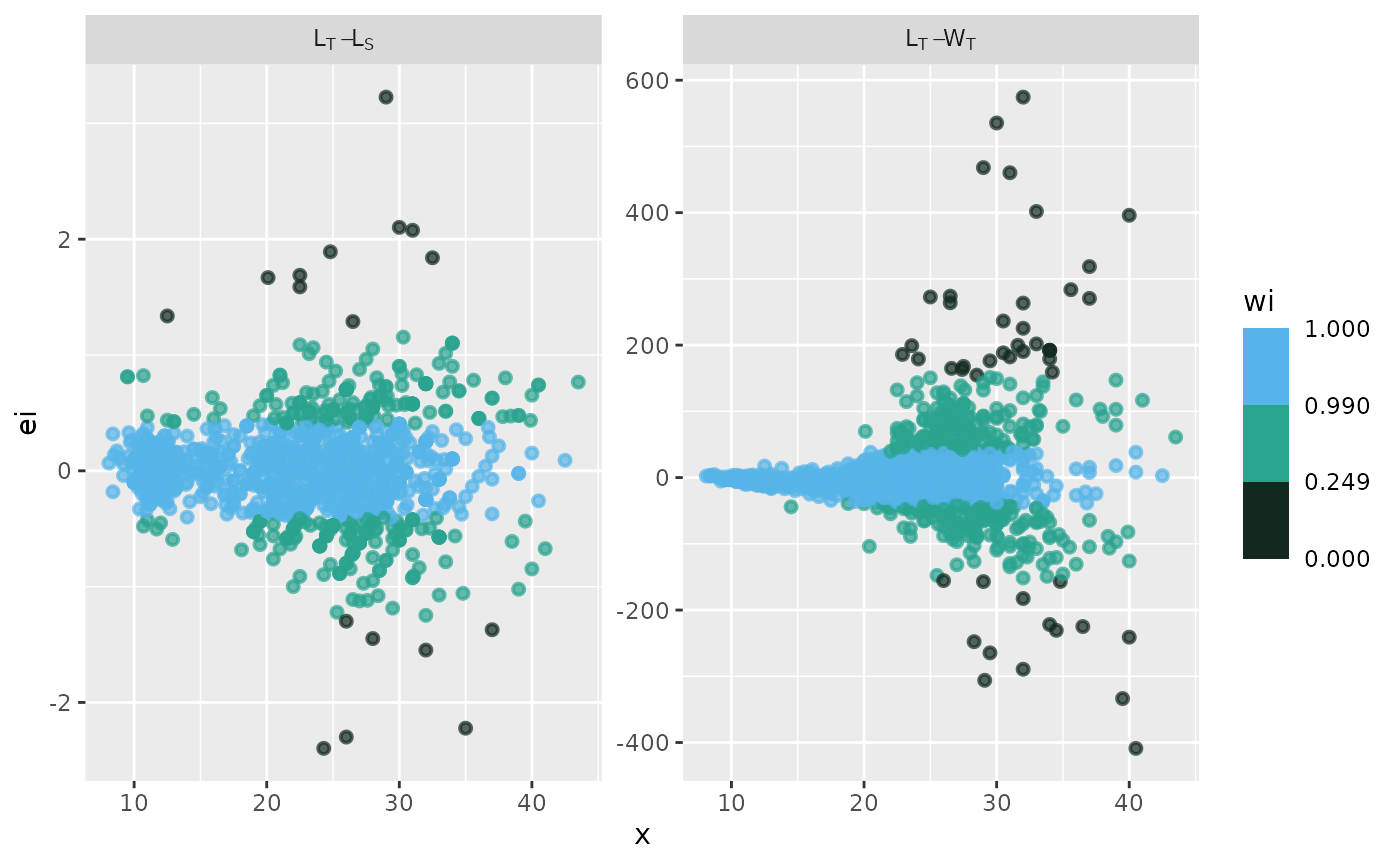

# theme papers()
p + theme_papers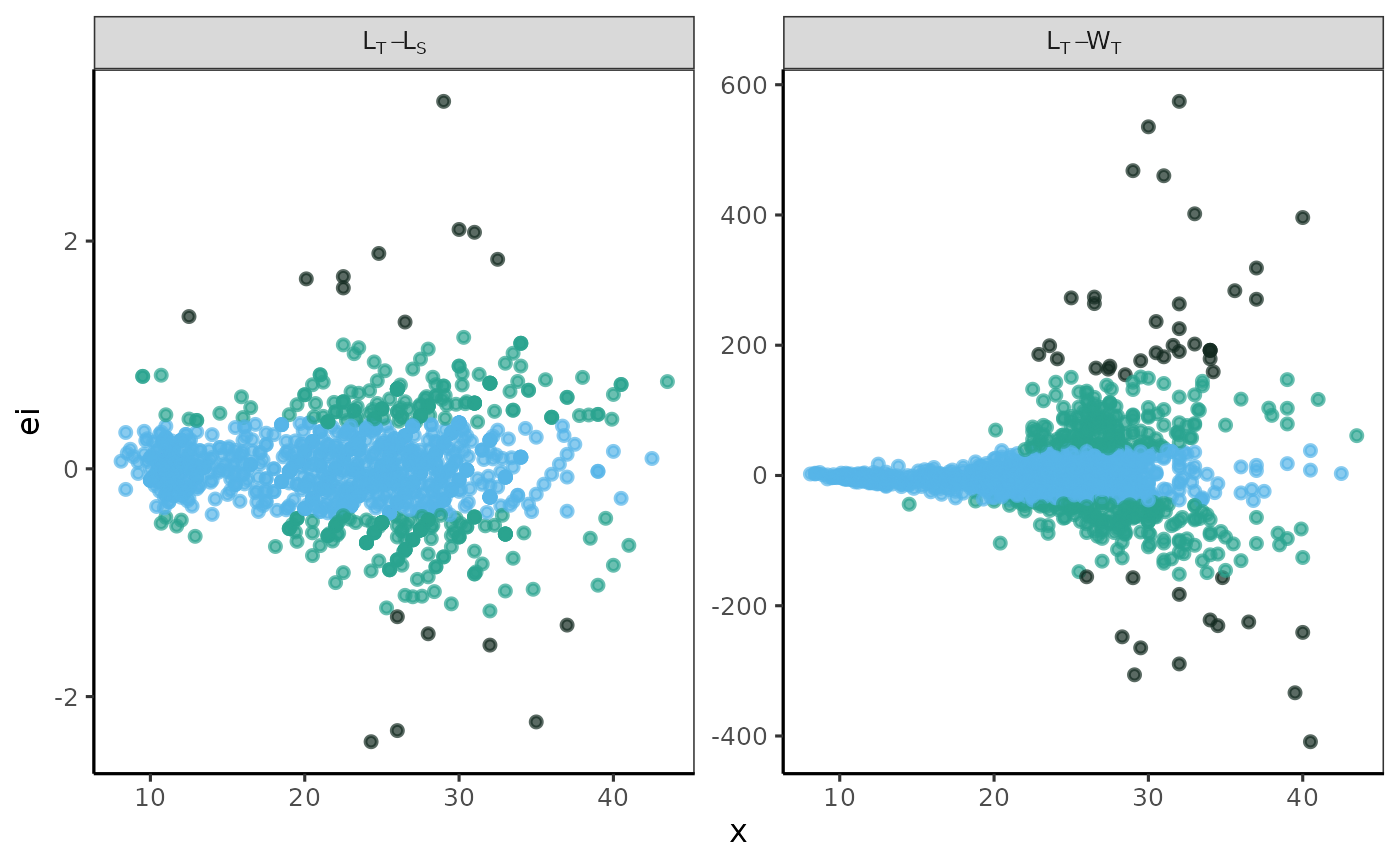

fn_fig_fw()

The fitted values of the models for a landed presentation category were displayed as a multi-panel plot. The observed data points for each fitted relationship were categorized according to a weighted color scale.

Example

The label in the grey box indicates the variables used for each model; the first variable listed is the independent variable, and the second is the dependent variable. The x-axis represents the values of the independent variable, while the y-axis displays the raw residuals (ei).

The standard graphical output, along with the one customized using the theme papers() function, is displayed.

# standard graphical output
p <- fn_fig_fw(df, opacity, tint, scale= wi_scale,
               order= X_names, my_labeller)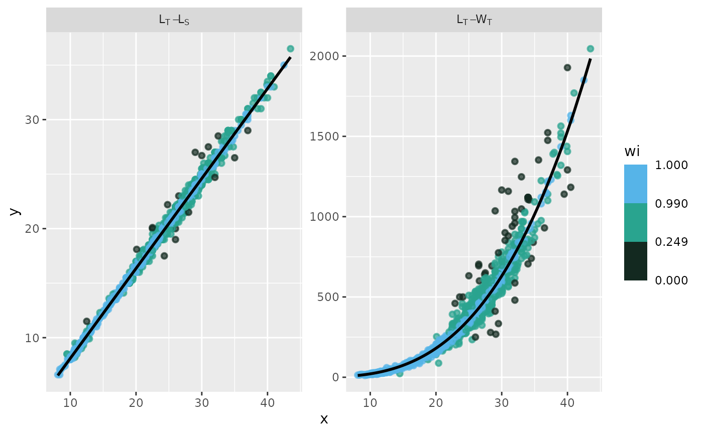

# theme papers()
p + theme_papers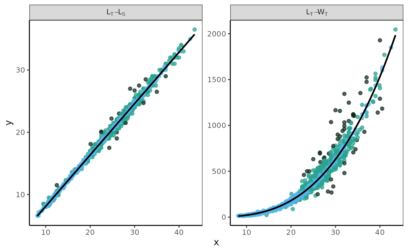

fn_fig_w()

The residual structure was analyzed by graphing residuals against weighted values. A custom multi-panel plot illustrates the structure of each fitted relationship, categorized by a color-weighted scale of values.

Example

The Residual Structures classified by a Weighted Scale was analyzed using combined data sets for the pufferfish Sphoeroides annulatus. The label in the grey box indicates the variables used for each model; the raw residuals are shown on the x-axis, and the weighted residuals (wi) are displayed on the y-axis.

The standard graphical output, along with the one customized using the theme papers() function, is displayed.

# standard graphical output
p <- fn_fig_w(df, opacity,tint, my_labeller,
              order= X_names)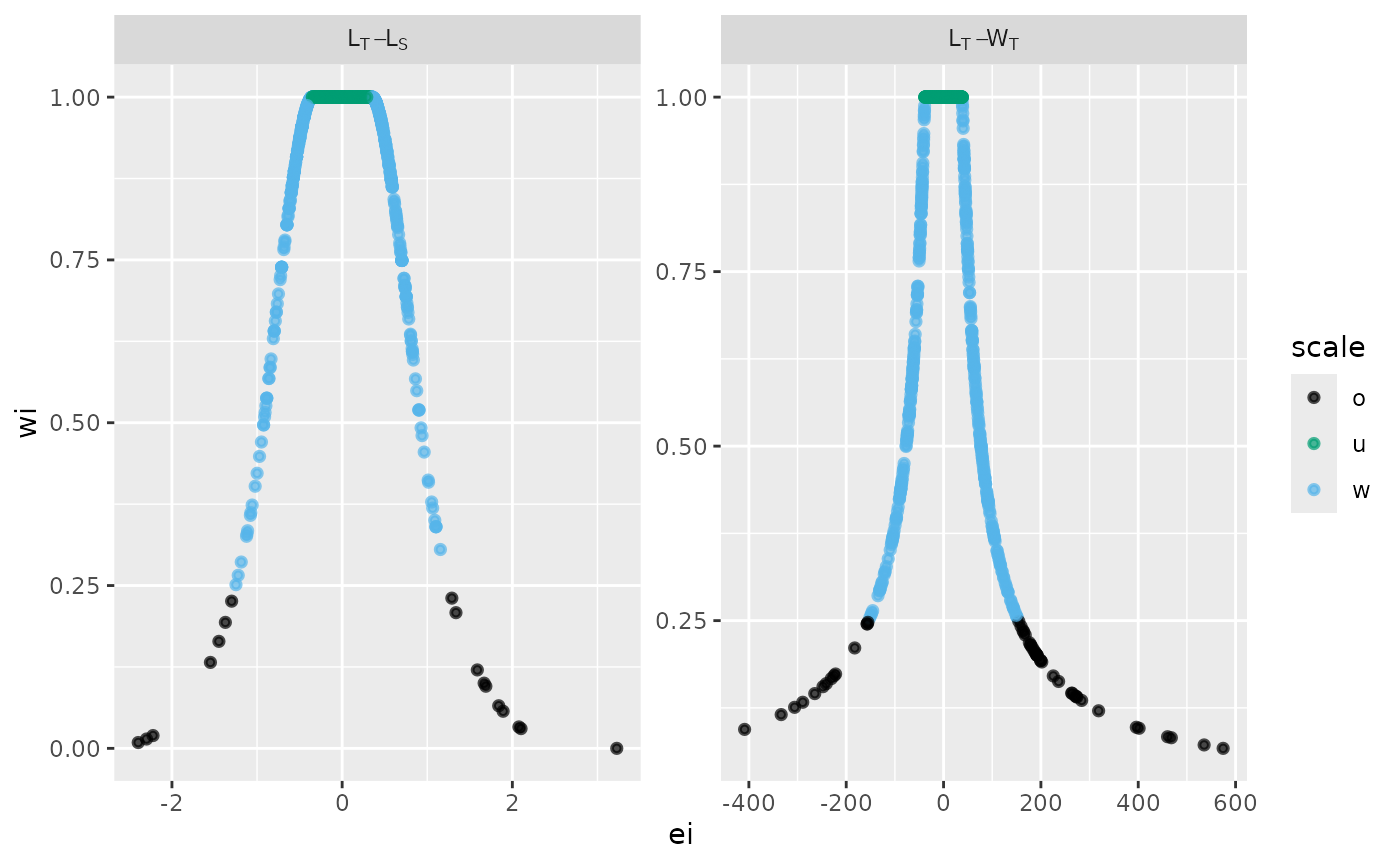

# theme papers()
p + theme_papers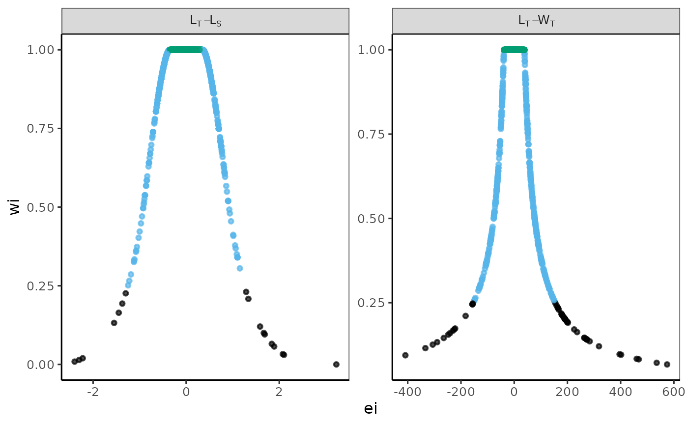

References

Chen, Y., Jackson, D. A., Harvey, H. H. 1992. A comparison of von Bertalanffy and polynomial functions in modelling fish growth data. Canadian Journal of Fisheries and Aquatic Sciences 49(6): 1228–1235. https://doi.org/10.1139/f92-13

Maechler M, Rousseeuw P, Croux C, Todorov V, Ruckstuhl A, Salibian-Barrera M, Verbeke T, Koller M, Conceicao EL, Anna di Palma M (2024). robustbase: Basic Robust Statistics. R package version 0.99-4-1, http://robustbase.r-forge.r-project.org/.

Renaud, O., Victoria-Feser, M. P. (2010). A robust coefficient of determination for regression. Journal of Statistical Planning and Inference. 140(7), 1852-1862. doi: 10.1016/j.jspi.2010.01.008.

SIPESCA. 2024. Sistema de Información de Pesca y Acuacultura – SIPESCA. Comisión Nacional de Pesca y Acuacultura. https://sipesca.conapesca.gob.mx (accessed 7 February 2024).

Esto no lo se Rick

# First hierarchical level: Models
    X_list <- vector(mode='list', length=2)
    X_names <- c("LT_LS", "LT_WT")
    names(X_list) <- X_names 
# Second hierarchical level: Category
    Fresh <- X_list
    Frozen <- X_list
    Total <- X_list
# Third hierarchical level: 
    List_fit <- list(Fresh,Frozen,Total) # Fitting results
    List_ICmodels <- List_fit # Confidence interval of the models.

List to store Coincident Curves Test Tables.

To store the results of each model regressions, an empty matrix of 4 rows and 8 columns are created. The table CCT stores the values and calculus for the Coincident Curves Test between weight categories: Fresh, Frozen, Total and Joined (sum of values of Fresh, Frozen): the residual sum of squares RSS, degree of freedom DF, Analysis of the Residual Sum of Squares ARSS, F-table, p-value and decision criteria for $\alpha$ = 0.05 Criteria.

To store the results of each fitted model, a list called List_TCCT was created. Each item in the list contains the customized table CCT, which is initially filled with NA values.

             
CCT <- (matrix(NA,nrow=4,ncol=8))
CCT[,2] <-  c("Fresh","Frozen","Total","Joined")
colnames(CCT) <- c("Model","Data","RSS","DF","ARSS","F-table",
                   "p-value","Criteria")

# Create model list including empty T1 table
List_TCCT <- setNames(lapply(1:length(modelos), function(x)
CCT),names(modelos))

CCT

List to store summary regression tables.

To store the summary regression, a customised table T1 is generated. The type of function model (Linear or Potential), and its variables, are indicated in the first two columns. The third column indicates the data source used (Fresh, Fresh-Thawed, or Total). By row it is stored: the Intercept, its confidence interval (CI95%); the Slope; its (CI95%); the adjusted robust coefficient of determination R2,adj,w,a and the degrees of freedom DF.

    # An empty table to store the summary regression results   
 
T1 <- data.frame(matrix(NA, nrow = 3, ncol = 9))
names(T1) <- c("Function", "Model","Categories",
               "Intercept", "CI95%","Slope",
               "CI95%", "R2","DF")
# Create model list including empty T1 table
List_Tables <- setNames(lapply(1:length(modelos), function(x)
T1),names(modelos))

T1
#>   Function Model Categories Intercept CI95% Slope CI95% R2 DF
#> 1       NA    NA         NA        NA    NA    NA    NA NA NA
#> 2       NA    NA         NA        NA    NA    NA    NA NA NA
#> 3       NA    NA         NA        NA    NA    NA    NA NA NA

Fitting modeles

Both relationships are fitted for the landed categories: Fresh, Frozen-thawed (Frozen), Total (All samples).

In the for loop, the jth landed categories is selected: 1 for Fresh, 2 for Frozen-thawed, 3 for the total sample.

# for (j in 1:3) {
#       if (j <3)  {
#             tmp <- mydata[mydata$Fleet == j,]
#             df <- dplyr::tibble(x1 = tmp[,1],y1 = tmp[,2])
#             # Fitting model
#             eq <- robustbase::lmrob(y1 ~ x1, data= df,
#                                      setting = "KS2014",
#                                      doCov = TRUE)
#             # Storing values
#             # Estimate confidence interval function
#           List_ICmodels[[j]][[1]] <- Morefi::fn_intervals(eq,xseq)
#           List_fit [[j]][[1]] <- fn_dfa(eq= eq)
#             
#             
#                 
#                 
#                 
#                 
#         }else{
#                 tmp <- mydata
#       } # End if
#   
#       df <- dplyr::tibble(x1 = tmp[,1],
#                 y1 = tmp[,2])
# 
# eq1 <- robustbase::lmrob(y1 ~ x1, data= df,
#                                   setting = "KS2014",
#                                               doCov = TRUE)
# 
# 
# 
# 
# 
# #  Power Model
# df <- dplyr::tibble(x1 = tmp[,1],
#                 y1 = tmp[,4])
# 
# a=0.01
# b=3
# 
# eq2 <- robustbase::nlrob(y1 ~ a*x1^b, data= df,
#                         start = list(a= a, b= b),
#                         trace = FALSE)
# 
#   
#   
#   
#   
#         # In the for loop, the ith model is selected.
# 
#     
#    # Linnear equation
#           eq <- robustbase::lmrob(y1 ~ x1, data= datos,
#                                   setting = "KS2014",
#                                               doCov = TRUE)
#     # R squared
#           R2 <- summary(eq)$r.squared    
#           #Non parametric IC 95 for parameters
#           betas_IC95 <- confint(eq, level = 0.95)
# 
#       }

Morefi

09 July 2025

Morefi: Example Analysis

Installation

Data available in the package

Bullseye puffer measures

Bullseye puffer fish landings

theme_papers()

Values to define for the examples

List: xseq

List: modelos

Morefi functions

Analysis functions

fn_ARSS()

Example

fn_dfa()

Example

fn_freq()

fn_freqw()

Example

fn_xseq()

Example

fn_intervals()

Example

fn_fyield()

Example

fn_R2RV()

Example

fn_summary()

fn_Wlive()

Plot functions

fn_fig_e()

Example

fn_fig_fw()

Example

fn_fig_w()

Example

References

Esto no lo se Rick

List to store Coincident Curves Test Tables.

List to store summary regression tables.

Fitting modeles

Aqui termina esto no lo sé Rick

`fn_freq()`